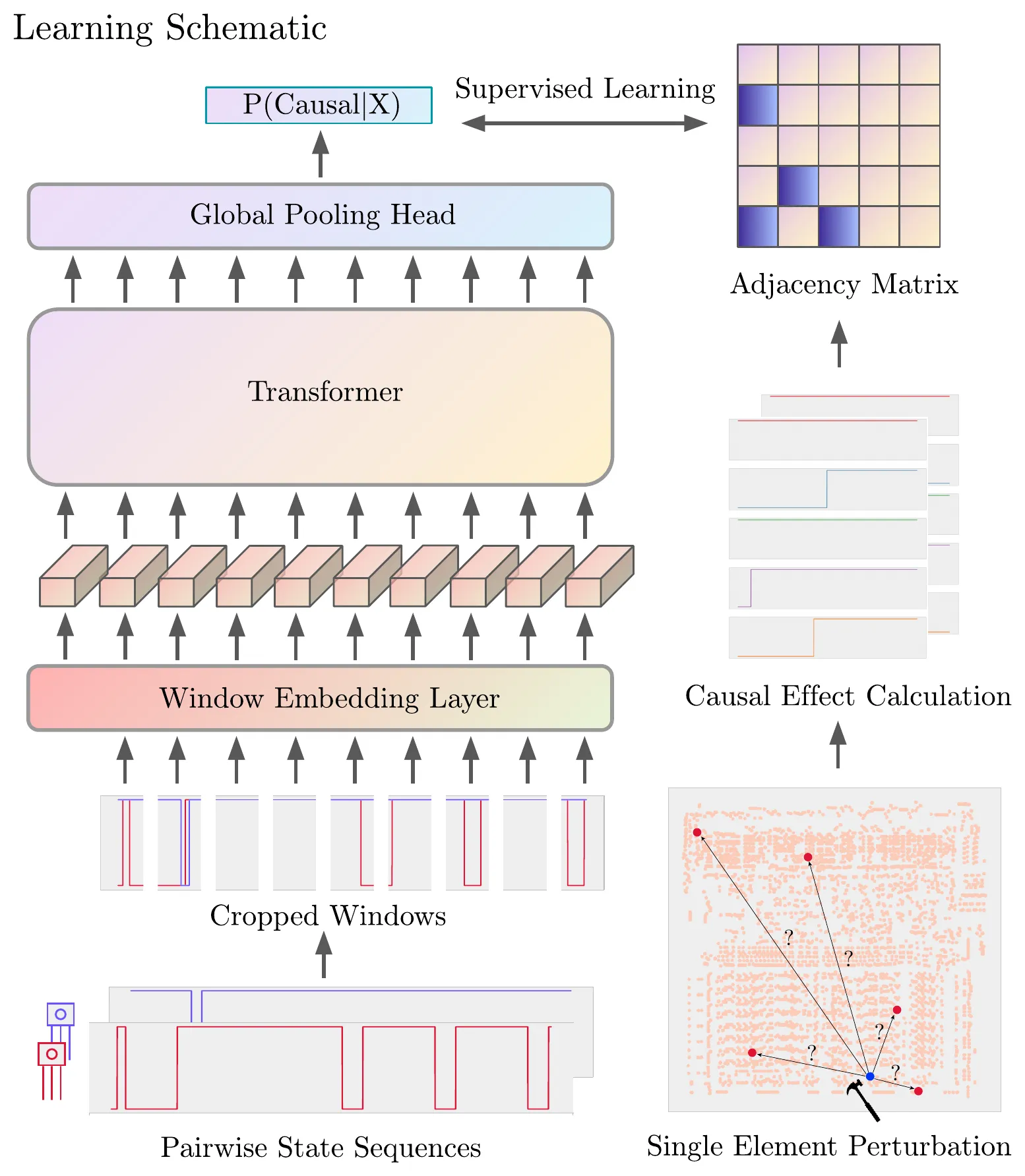
To learn causal discovery you need a system where every true cause-and-effect relationship is already known — and no brain, economy or cell will give you that. A microprocessor will. Perturb any transistor in simulation, watch what changes downstream, and the ground truth falls out. So rather than designing a causal discovery algorithm, we learned one, on a MOS 6502 running Donkey Kong.
The bet
Classical causal discovery encodes human assumptions. Granger causality, conditional-independence tests, structural equation models, score-based search — each is accurate exactly where its assumptions hold, and each was designed by a person reasoning about what a causal system ought to look like.
Everywhere else in machine learning, hand-designed features eventually lost to learned ones once data became abundant. The question this work asks is whether causal discovery is any different: can the discovery procedure itself be learned from data?
The paper’s answer is a thesis about the field, not just a method — that where it is feasible, we should learn domain-specific causal discovery procedures from large datasets with known causal relationships, rather than have specialists design them.
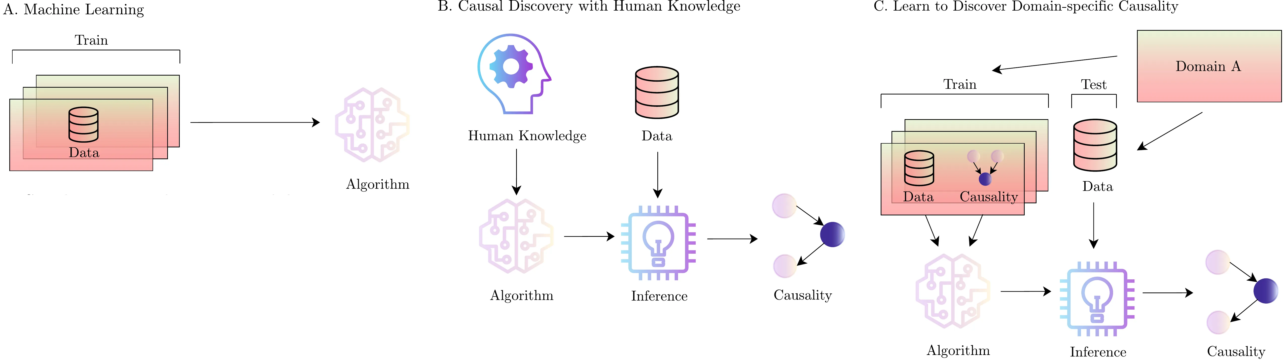 Three ways to get a causal estimator. (A) In machine learning, estimators are learned from data. (B) In traditional causal discovery, the estimator is a human-designed algorithm and the data is only checked against its assumptions. (C) This work: learn a domain-specific estimator from observations paired with known causality.
A system where ground truth is knowable
The MOS 6502 has 3,510 transistors wired into multi-input, multi-output connections. A C++ simulator runs three game recordings — Donkey Kong, Pitfall and Space Invaders — while every transistor’s state is sampled 30 times within each half-clock.
Ground truth comes from intervention. Perturb a single transistor at the midpoint of a recording period, re-run, and measure the expected absolute difference in every other transistor’s trace. Any non-zero difference is a causal edge. Crucially, the effect is computed only over the first half-clock after the perturbation, which keeps the measured relations relatively direct rather than letting influence cascade through the whole chip. Repeating this for every transistor across 320 periods produces the labelled corpus.
The line that justifies the entire exercise is this: the wiring diagram is not the causal graph. A netlist for the 6502 exists, but it carries no direction — nothing distinguishing cause from effect, and no account of how influence actually flows through multi-input connections. The demonstration is concrete: perturbing transistor 134 changes nothing downstream, despite the physical wires leaving it.
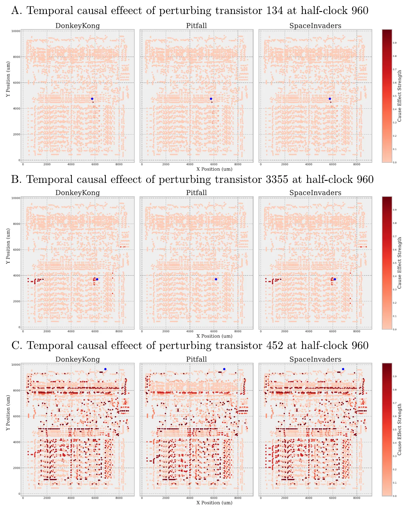 One perturbation, three programs. Each panel is the physical layout of the chip; the blue dot is the perturbed transistor and red marks everything it causally affects. Perturb transistor 452 and most of the chip lights up — one of its downstream transistors feeds the clock line that synchronizes everything. A causal footprint turns out to track functional importance.
Two further facts shape the problem. The first is that causality is rare — roughly 300 causal pairs among some 36,000 transistor pairs. This is why average precision, not ROC, is the metric that matters here: with 1% positives, a flattering ROC curve is easy and nearly meaningless.
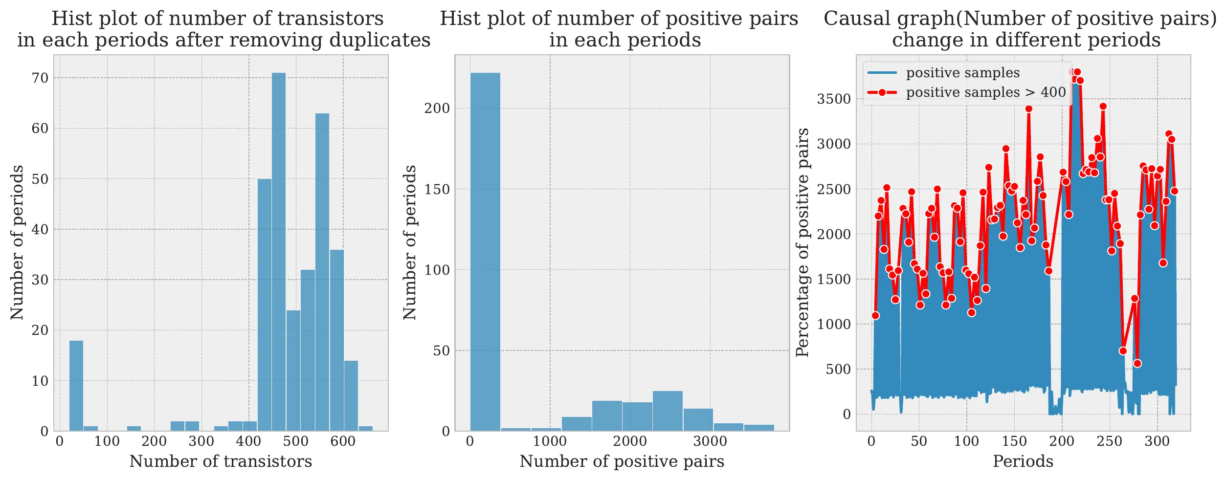 Causality is rare, and unevenly distributed. Unique transistors and positive (causal) pairs across recording periods. Periods with unusually many causal pairs recur at a regular interval.
The second is that the graph is non-stationary. Perturbing the same transistor at different moments yields completely different effect maps — partly because the video chip that talks to the CPU is never modelled, and acts as a hidden confounder inside the benchmark itself.
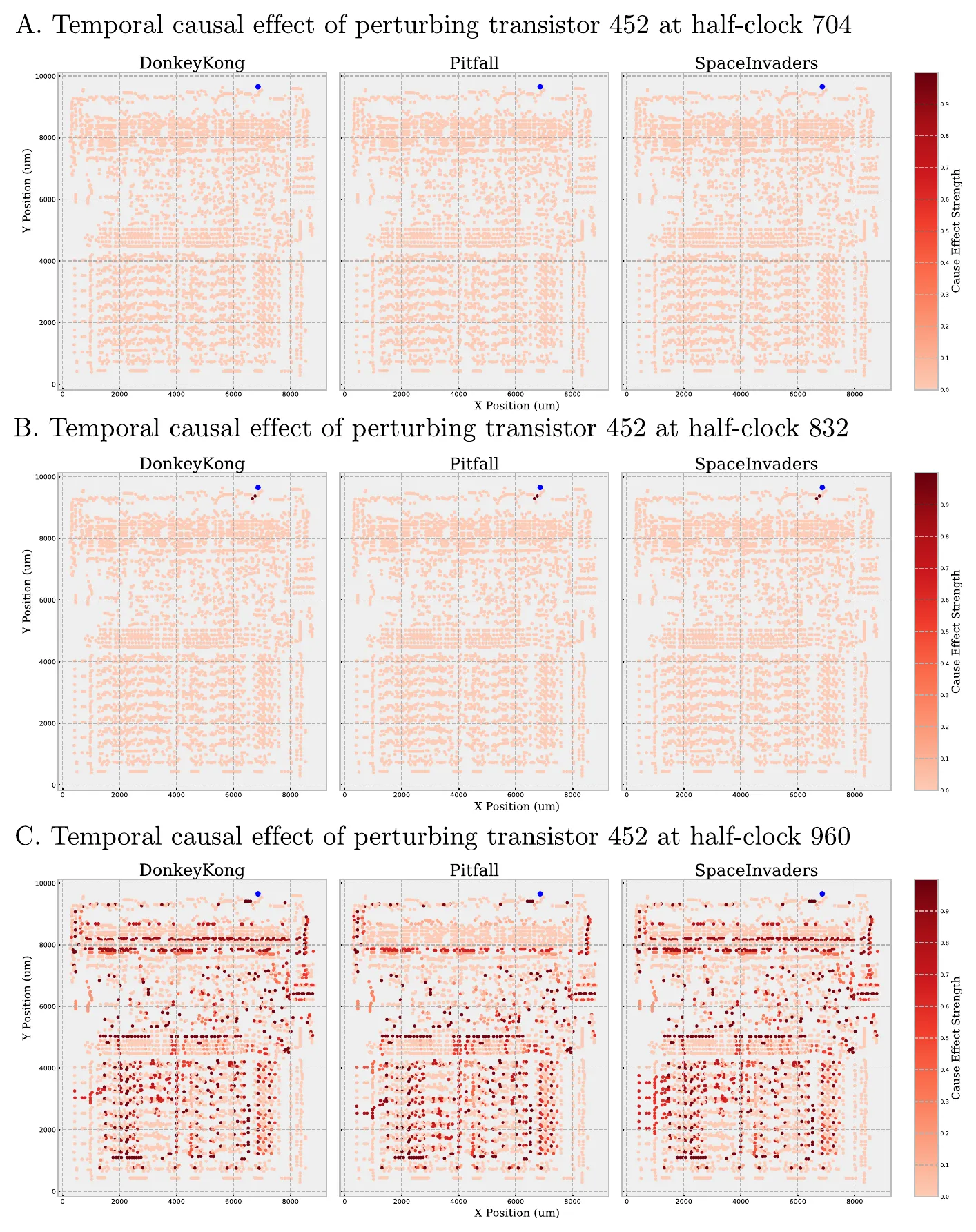 The causal graph is not static. The same transistor perturbed at three different half-clocks. A single fixed graph is the wrong model for a system that is still running.
What the model actually sees
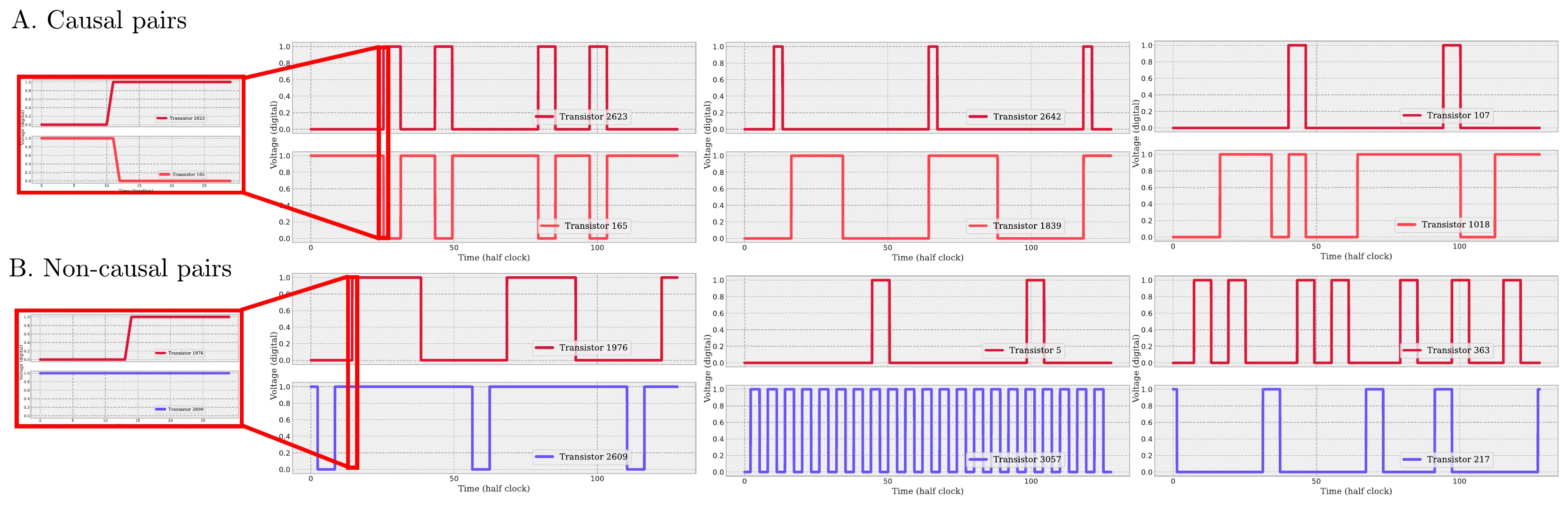 Which of these pairs is causal? Six pairs of transistor voltage traces — three causal (top), three not (bottom), with the lag visible only in the zoomed inset. This is the entire input: two sequences, no graph, no metadata.
A sample is a pair of time series stacked into a single array, labelled by one entry of the adjacency matrix. Because the pair is ordered, and are different samples — direction is something the model has to learn, not something the representation assumes.
The sequences are long and mostly flat, with far more constant stretches than informative transitions. So the model crops them into non-overlapping windows, embeds each window with a 1-D convolution, prepends a class token and runs a transformer across windows, then pools with attention — the pooling is what lets it weight the few windows where anything actually happens.
One property is worth emphasizing: perturbation is used only to create training labels. At inference the estimator is purely observational, and because its input is a pair rather than a full system, it can be applied to systems with any number of nodes.
Results
Testing is deliberately unforgiving: the estimator is trained on the first half of the transistors and evaluated on the other half, in held-out time periods.
On Donkey Kong it reaches 0.48 ± 0.10 AUPRC and 0.97 ± 0.03 AUROC. On identical inputs, correlation — the tool most often reached for when people discuss connectivity — manages about 0.13 AUPRC, and mutual information, VAR-LiNGAM and Granger causality all land in the same band.
Zero-shot across programs. The estimator is trained only on Donkey Kong. Applied to two other games with no retraining, it barely notices: same silicon, different software, different dynamics, and the learned notion of causality carries over intact.
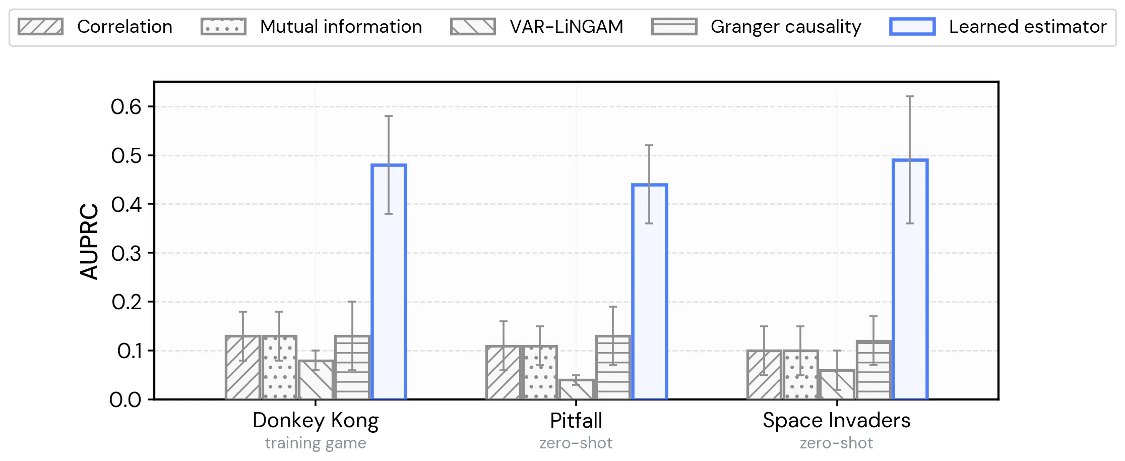 Average precision on held-out transistors and held-out time. The learned estimator is roughly four times the best classical method, and the two zero-shot games are indistinguishable from the one it trained on. Bars are means over five test periods; whiskers are one standard deviation.
Simulated fMRI. Trained on five NetSim simulations and evaluated on sixteen with different node counts and system properties, the estimator reaches 0.85–0.99 AUPRC on fourteen of seventeen simulations, while every classical and neural baseline — DYNOTEARS, PCMCI+, VAR-LiNGAM, neural Granger, eSRU and SRU among them — stays below 0.5. It fails on the three most out-of-distribution simulations, and the paper says so.
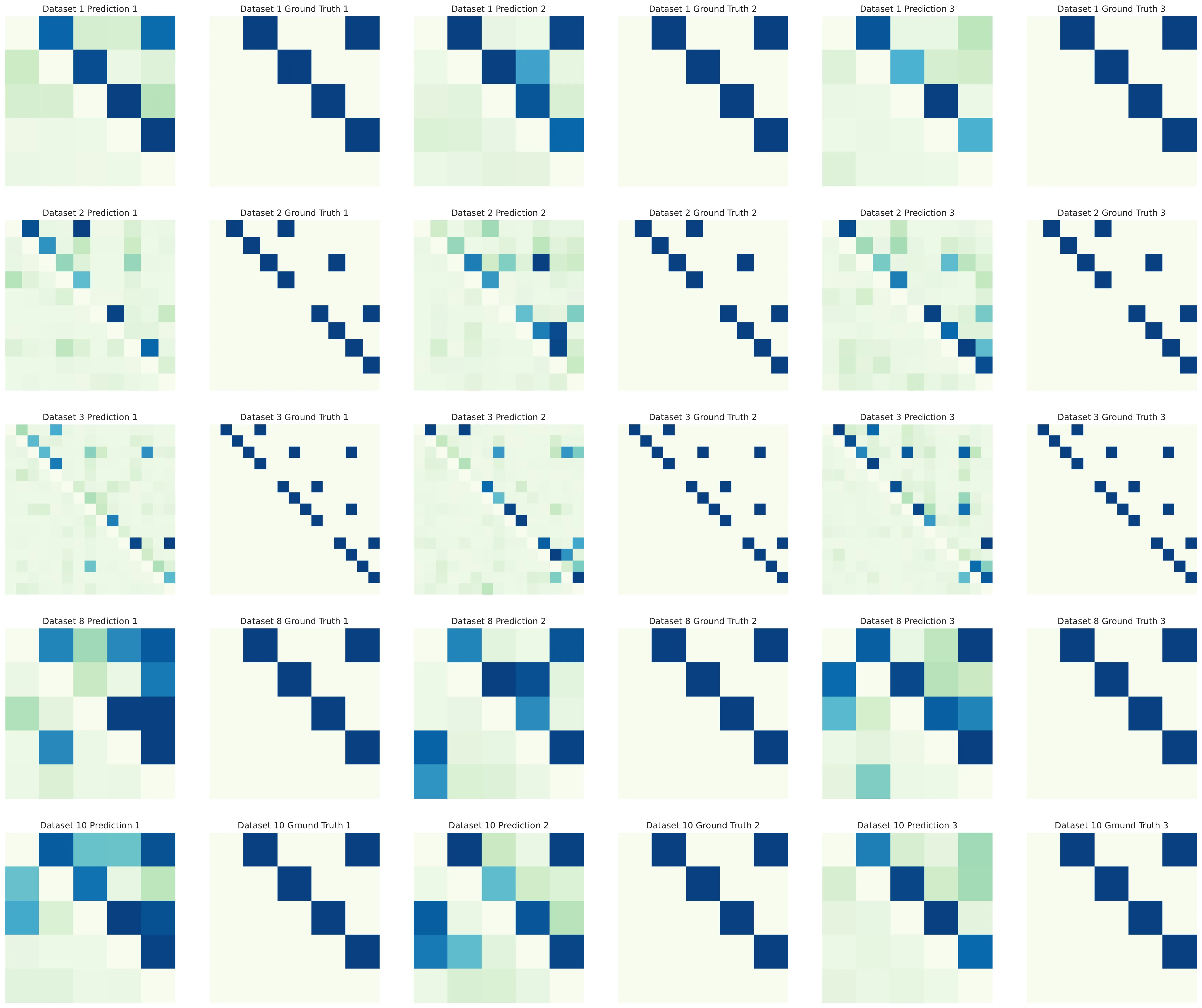 Recovered connectivity on simulated fMRI. Inferred P(causal | X) matrices beside the ground-truth connection matrices, for simulations the estimator was never trained on.
One clarification, because the framing invites a misreading: there is no microprocessor-to-brain transfer here. A separate estimator is trained per domain. What generalizes is the approach, plus a genuinely broad within-domain robustness — unseen transistors, unseen time periods, unseen programs and added noise.
Did it learn causality, or a shortcut?
A supervised model that scores well on a benchmark invites the obvious suspicion. Two checks push back.
Where it looks. Gradient saliency over the last attention block concentrates precisely on the windows where cause and effect interact — the handful of transitions in an otherwise flat trace — and keeps doing so when noise is added.
See the gradient saliency analysis
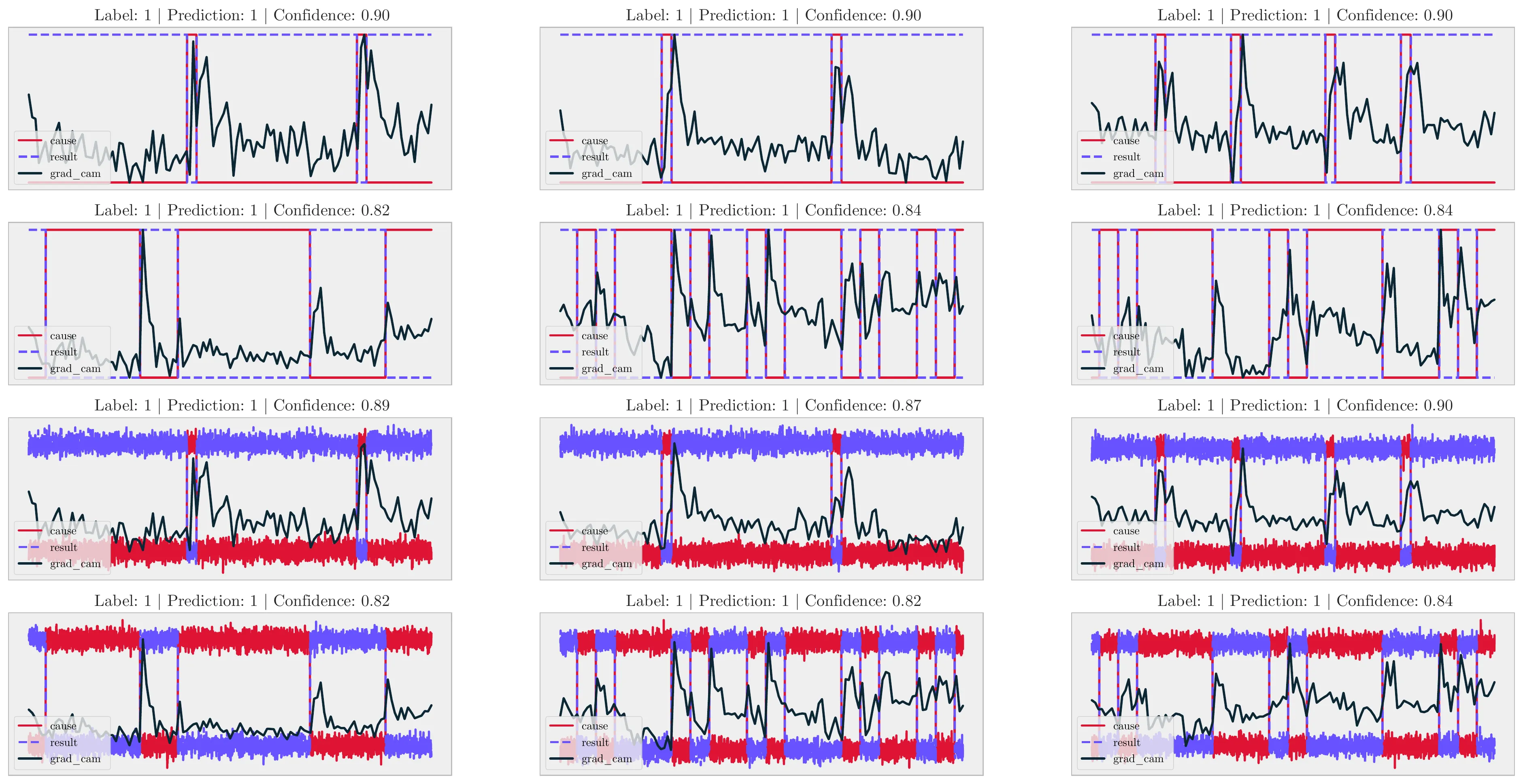 Where the model looks. Gradient saliency for three causal pairs, in the clean setting (top) and with added observational noise (bottom). Attention concentrates at the transitions — the only places causal information exists.
The arrow of time. Shift the effect trace backwards by one half-clock, so the effect now precedes its cause, and the model reverses its verdict: confidence in causality collapses to roughly 0.2 and the prediction flips to “not causal.” Nothing in the training objective mentioned temporal precedence. It was learned.
See the temporal reversal experiment
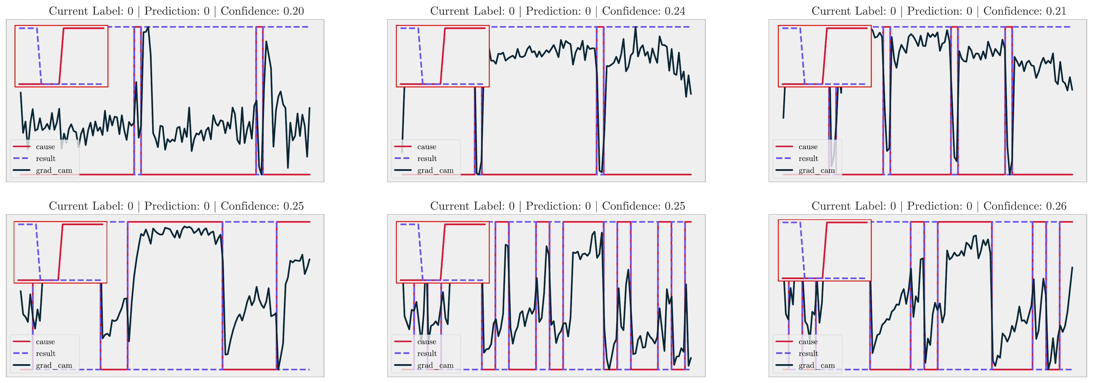 Breaking the arrow of time. The same pairs the model confidently called causal, with the effect shifted to precede the cause. Confidence collapses and every prediction flips.
Where it breaks
Noise. Robust through a noise scale of 0.1, degraded at 0.3, and at 0.5 it is beaten by plain correlation. Enough noise buries the pattern the estimator was trained to see.
Small samples. On Dream3 gene networks — roughly 270 positive pairs among 10,000 samples — AUPRC collapses to 0.04–0.06 and training overfits almost immediately. Learned causal discovery needs a supervised corpus, and that corpus needs to be big.
A local view. Pairwise input means no global, multivariate perspective on the graph. It is the direct cost of the property that lets the same estimator run on systems of any size.
It presumes ground truth exists. Which is the honest reason a microprocessor was chosen at all: neither medicine nor neuroscience currently has large observational datasets paired with perturbation-derived causal ground truth.
What it argues for
That last limitation is really the proposal. Public policy and medicine already run thousands of real perturbations every year — tax changes, regulatory exemptions, new drugs, revised clinical guidelines. Each one is an intervention with a recorded before and after.
If those were assembled the way the 6502 corpus was assembled, the same recipe would apply: learn the discovery procedure from the domain instead of importing assumptions into it. The chip is a proof of concept for a claim about where causal discovery should get its knowledge from.